6. Differential Gene expression and GO enrichment from RNA-Seq data

Differential expression (DE) analysis allows the comparison of RNA expression levels between multiple conditions.

The differential gene expression and GO enrichment pipeline is comprised of five steps, shown in next Table. The first step involves downloading samples from the NCBI SRA database, if necessary, or executing the pre-processing quality control tools on local samples. Subsequently, sample trimming, alignment, and quantification processes are executed. Once all samples are processed, groups of differentially expressed genes are identified per condition, using DESeq and EdgeR. Over- and under-expressed genes are reported by each program, and the interception of their results is computed.

Finally, once differentially expressed genes are identified, a GO enrichment analysis is executed to provide key biological processes, molecular functions, and cellular components for identified genes.

DGA and Go enrichment, RNASeq pipeline

Step	Jupyter Notebook	Workflow CWL	Tool	Input	Output	CWL Tool
Sample Download and Quality Control	01 - Pre-processing QC	download_quality_control.cwl	SRA-Tools	SRA accession	Fastq	fastq-dump.cwl
			FastQC	Fastq	FastQC HTML and Zip	fastqc.cwl
Trimming	02 - Samples trimming		Trimmomatic	Fastq	Fastq	trimmomatic-PE.cwl trimmomatic-SE.cwl
Alignments and Quantification	03 - Alignments and Quantification	rnaseq-alignment-quantification.cwl	STAR	Fastq	BAM	star.cwl
			Samtools	SAM	BAM Sorted BAM BAM index BAM stats BAM flagstats	samtools-view.cwl samtools-sort.cwl samtools-index.cwl samtools-stats.cwl samtools-flagstat.cwl
			IGVtools	Sorted BAM	TDF	igvtools-count.cw
			RSeQC	Sorted BAM	Alignment quality control (TXT and PDF)	rseqc-bam_stat.cwl rseqc-infer_experiment.cwl rseqc-junction_annotation.cwl rseqc-junction_saturation.cwl rseqc-read_distribution.cwl rseqc-read_quality.cwl
			TPMCalculator	Sorted BAM	Read counts (TSV) TPM values (TSV)	tpmcalculator.cwl
Differential Gene Analysis	04 - DGA		DeSEq2	Read Matrix	TSV	deseq2-2conditions.cwl
			EdgeR	Read Matrix	TSV	edgeR-2conditions.cwl
Go enrichment	05 - GO enrichment		goenrichment	gene IDs	TSV	Python code in the notebook

6.1. Input requirements

The input requirement for the DGA pipeline is the Sample sheet file.

6.2. Pipeline command line

The RNASeq based project can be created using the following command line:

localhost:~> pm4ngs-rnaseq
usage: Generate a PM4NGS project for RNA-Seq data analysis [-h] [-v]
                                                       --sample-sheet
                                                       SAMPLE_SHEET
                                                       [--config-file CONFIG_FILE]
                                                       [--copy-rawdata]

Options:

• sample-sheet: Sample sheet with the samples metadata
• config-file: YAML file with configuration for project creation
• copy-rawdata: Copy the raw data defined in the sample sheet to the project structure. (The data can be hosted locally or in an http server)

6.3. Creating the DGA and GO enrichment from RNA-Seq data project

The pm4ngs-rnaseq command line executed with the --sample-sheet option will let you type the different variables required for creating and configuring the project. The default value for each variable is shown in the brackets. After all questions are answered, the CWL workflow files will be cloned from the github repo ncbi/cwl-ngs-workflows-cbb to the folder bin/cwl.

localhost:~> pm4ngs-rnaseq --sample-sheet my-sample-sheet.tsv
Generating RNA-Seq data analysis project
author_name [Roberto Vera Alvarez]:
email [veraalva@ncbi.nlm.nih.gov]:
project_name [my_ngs_project]:
dataset_name [my_dataset_name]:
is_data_in_SRA [y]:
Select sequencing_technology:
1 - single-end
2 - paired-end
Choose from 1, 2 [1]: 2
create_demo [y]: y
number_spots [1000000]:
organism [human]:
genome_name [hg38]:
genome_dir [hg38]:
aligner_index_dir [hg38/STAR]:
genome_fasta [hg38/genome.fa]:
genome_gtf [hg38/genes.gtf]:
genome_bed [hg38/genes.bed]:
fold_change [2.0]:
fdr [0.05]:
use_docker [y]:
max_number_threads [16]:
Cloning Git repo: https://github.com/ncbi/cwl-ngs-workflows-cbb to /home/veraalva/tmp/cookiecutter/my_ngs_project/bin/cwl
Updating CWLs dockerPull and SoftwareRequirement from: /home/veraalva/my_ngs_project/requirements/conda-env-dependencies.yaml
bioconductor-diffbind with version 2.16.0 update image to: quay.io/biocontainers/bioconductor-diffbind:2.16.0--r40h5f743cb_0
    /home/veraalva/my_ngs_project/bin/cwl/tools/R/deseq2-pca.cwl with old image replaced: quay.io/biocontainers/bioconductor-diffbind:2.16.0--r40h5f743cb_2
    /home/veraalva/my_ngs_project/bin/cwl/tools/R/macs-cutoff.cwl with old image replaced: quay.io/biocontainers/bioconductor-diffbind:2.16.0--r40h5f743cb_2
    /home/veraalva/my_ngs_project/bin/cwl/tools/R/dga_heatmaps.cwl with old image replaced: quay.io/biocontainers/bioconductor-diffbind:2.16.0--r40h5f743cb_2
    /home/veraalva/my_ngs_project/bin/cwl/tools/R/diffbind.cwl with old image replaced: quay.io/biocontainers/bioconductor-diffbind:2.16.0--r40h5f743cb_2
    /home/veraalva/my_ngs_project/bin/cwl/tools/R/edgeR-2conditions.cwl with old image replaced: quay.io/biocontainers/bioconductor-diffbind:2.16.0--r40h5f743cb_2
    /home/veraalva/my_ngs_project/bin/cwl/tools/R/volcano_plot.cwl with old image replaced: quay.io/biocontainers/bioconductor-diffbind:2.16.0--r40h5f743cb_2
    /home/veraalva/my_ngs_project/bin/cwl/tools/R/readQC.cwl with old image replaced: quay.io/biocontainers/bioconductor-diffbind:2.16.0--r40h5f743cb_2
    /home/veraalva/my_ngs_project/bin/cwl/tools/R/deseq2-2conditions.cwl with old image replaced: quay.io/biocontainers/bioconductor-diffbind:2.16.0--r40h5f743cb_2
Copying file /home/veraalva/Work/Developer/Python/pm4ngs/pm4ngs-rnaseq/example/pm4ngs_rnaseq_demo_sample_data.csv  to /Users/veraalva/my_ngs_project/data/my_dataset_name/sample_table.csv
20 files loaded
Using table:
   sample_name file       condition  replicate
0   SRR2126784             PRE_NACT          1
1   SRR2126785             PRE_NACT          1
2   SRR2126786             PRE_NACT          1
3   SRR2126787             PRE_NACT          1
4   SRR3383790             PRE_NACT          1
5   SRR3383791             PRE_NACT          1
6   SRR3383792             PRE_NACT          1
7   SRR3383794             PRE_NACT          1
8   SRR3383796             PRE_NACT          1
9   SRR3383797             PRE_NACT          1
10  SRR3383798             PRE_NACT          1
11  SRR2126788       POST_NACT_CRS3          1
12  SRR2126789       POST_NACT_CRS3          1
13  SRR2126790       POST_NACT_CRS3          1
14  SRR2126791       POST_NACT_CRS3          1
15  SRR2126792       POST_NACT_CRS3          1
16  SRR2126793       POST_NACT_CRS3          1
17  SRR2126794       POST_NACT_CRS3          1
18  SRR2126795       POST_NACT_CRS3          1
19  SRR2126796       POST_NACT_CRS3          1
 Done

The pm4ngs-rnaseq command line will create a project structure as:

.
├── LICENSE
├── README.md
├── bin
│   └── cwl
├── config
│   └── init.py
├── data
│   └── my_dataset_name
│       └── sample_table.csv
├── doc
├── index.html
├── notebooks
│   ├── 00 - Project Report.ipynb
│   ├── 01 - Pre-processing QC.ipynb
│   ├── 02 - Samples trimming.ipynb
│   ├── 03 - Alignments and Quantification.ipynb
│   ├── 04 - DGA.ipynb
│   └── 05 - GO enrichment.ipynb
├── requirements
│   └── conda-env-dependencies.yaml
├── results
│   └── my_dataset_name
├── src
└── tmp

61 directories, 239 files

Note

RNASeq based project variables

• author_name:

  Default: [Roberto Vera Alvarez]

• email:

  Default: [veraalva@ncbi.nlm.nih.gov]

• project_name:

  Name of the project with no space nor especial characters. This will be used as project folder's name.

  Default: [my_ngs_project]

• dataset_name:

  Dataset to process name with no space nor especial characters. This will be used as folder name to group the data. This folder will be created under the data/{{dataset_name}} and results/{{dataset_name}}.

  Default: [my_dataset_name]

• is_data_in_SRA:

  If the data is in the SRA set this to y. A CWL workflow to download the data from the SRA database to the folder data/{{dataset_name}} and execute FastQC on it will be included in the 01 - Pre-processing QC.ipynb notebook.

  Set this option to n, if the fastq files names and location are included in the sample sheet.

  Default: [y]

• Select sequencing_technology:

  Select one of the available sequencing technologies in your data.

  Values: 1 - single-end, 2 - paired-end

• create_demo:

  If the data is downloaded from the SRA and this option is set to y, only the number of spots specified in the next variable will be downloaded. Useful to test the workflow.

  Default: [y]: y

• number_spots:

  Number of sport to download from the SRA database. It is ignored is the create_demo is set to n.

  Default: [1000000]

• organism:

  Organism to process, e.g. human. This is used to link the selected genes to the NCBI gene database.

  Default: [human]

• genome_name:

  Genome name , e.g. hg38 or mm10.

  Default: [hg38]

• genome_dir:

  Absolute path to the directory with the genome annotation (genome.fa, genes.gtf) to be used by the workflow or the name of the genome.

  If the name of the genome is used, PM4NGS will include a cell in the 03 - Alignments and Quantification.ipynb notebook to download the genome files. The genome data will be at data/{{dataset_name}}/{{genome_name}}/

  Default: [hg38]

• aligner_index_dir:

  Absolute path to the directory with the genome indexes for STAR.

  If {{genome_name}}/STAR is used, PM4NGS will include a cell in the 03 - Alignments and Quantification.ipynb notebook to create the genome indexes for STAR.

  Default: [hg38/STAR]

• genome_fasta:

  Absolute path to the genome fasta file

  If {{genome_name}}/genome.fa is used, PM4NGS will use the downloaded fasta file.

  Default: [hg38/genome.fa]

• genome_gtf:

  Absolute path to the genome GTF file

  If {{genome_name}}/genes.gtf is used, PM4NGS will use the downloaded GTF file.

  Default: [hg38/gene.gtf]

• genome_bed:

  Absolute path to the genome BED file

  If {{genome_name}}/genes.bed is used, PM4NGS will use the downloaded BED file.

  Default: [hg38/genes.bed]

• fold_change:

  A real number used as fold change cutoff value for the DG analysis, e.g. 2.0.

  Default: [2.0]

• fdr:

  Adjusted P-Value to be used as cutoff in the DG analysis, e.g. 0.05.

  Default: [0.05]

• use_docker:

  Set this to y if you will be using Docker. Otherwise Conda needs to be installed in the computer.

  Default: [y]

• max_number_threads:

  Number of threads available in the computer.

  Default: [16]

6.4. Jupyter server

PM4NGS uses Jupyter as interface for users. After project creation the jupyter server should be started as shown below. The server will open a browser windows showing the project's structure just created.

localhost:~> jupyter notebook

6.5. Data processing

Start executing the notebooks from 01 to 05 waiting for each step completion. The 00 - Project Report.ipynb notebook can be executed after each notebooks to see the progress in the analysis.

6.6. CWL workflows

6.6.1. SRA download and QC workflow

This CWL workflow is designed to download FASTQ files from the NCBI SRA database using fastq-dump and then, execute fastqc generating a quality control report of the sample.

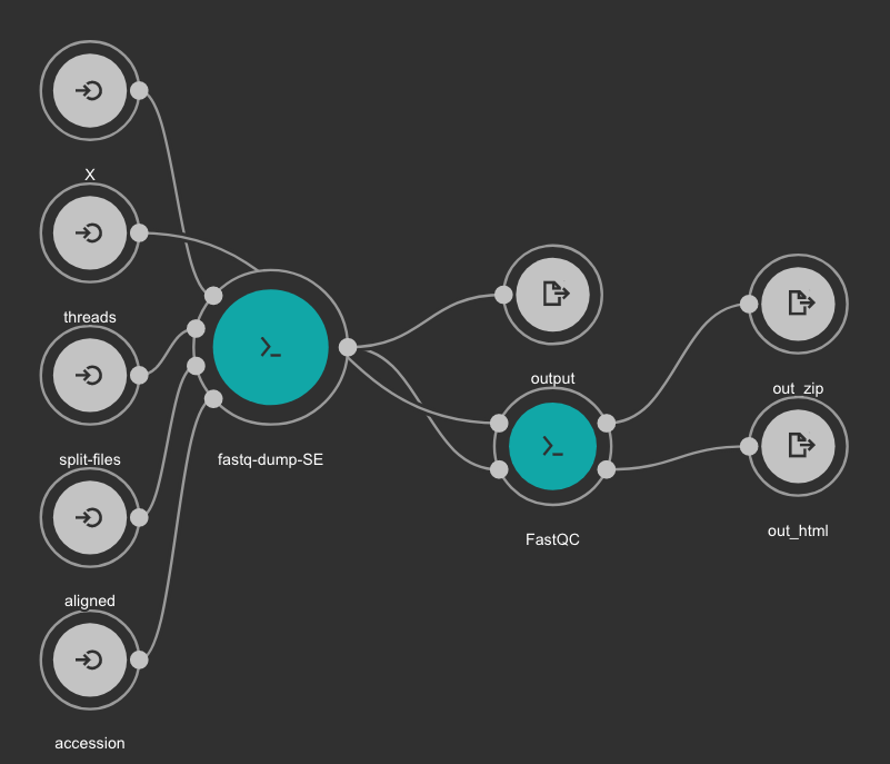
Inputs

• accession: SRA accession ID. Type: string. Required.
• aligned: Used it to download only aligned reads. Type: boolean. Optional.
• split-files: Dump each read into separate file. Files will receive suffix corresponding to read number. Type: boolean. Optional.
• threads: Number of threads. Type: int. Default: 1. Optional.
• X: Maximum spot id. Optional.

Outputs

• output: Fastq files downloaded. Type: File[]
• out_zip: FastQC report ZIP file. Type: File[]
• out_html: FastQC report HTML. Type: File[]

6.6.2. Samples Trimming

Our workflows uses Trimmomatic for read trimming. The Jupyter notebooks uses some basic Trimmomatic options that need to be modified depending on the FastQC quality control report generated for the sample.

6.6.3. STAR based alignment and sorting

This workflows use STAR for alignning RNA-Seq reads to a genome. The obtained BAM file is sorted using SAMtools. Statistics outputs from STAR and SAMtools are returned as well.

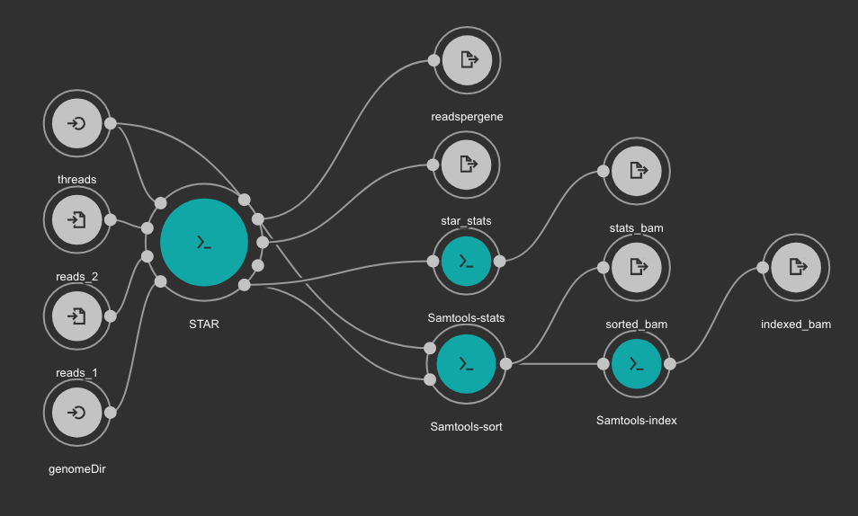
Inputs

• genomeDir: Aligner indexes directory. Type: Directory. Required. Variable ALIGNER_INDEX in the Jupyter Notebooks.
• threads: Number of threads. Type: int. Default: 1. Optional.
• reads_1: FastQ file to be processed for paired-end reads _1. Type: File. Required.
• reads_2: FastQ file to be processed for paired-end reads _2. Type: File. Required.

Outputs

• sorted_bam: Final BAM file filtered and sorted. Type: File.
• indexed_bam: BAM index file. Type: File.
• star_stats: STAR alignment statistics. Type: File.
• readspergene: STAR reads per gene output. Type: File.
• stats_bam: SAMtools stats output: Type: File.

6.6.4. RNA-Seq quantification and QC workflow using TPMCalculator

This workflow uses TPMCalculator to quantify the abundance of genes and transcripts from the sorted BAM file. Additionally, RSeQC is executed to generate multiple quality control outputs from the sorted BAM file. At the end, a TDF file is generated using igvtools from the BAM file for a quick visualization.

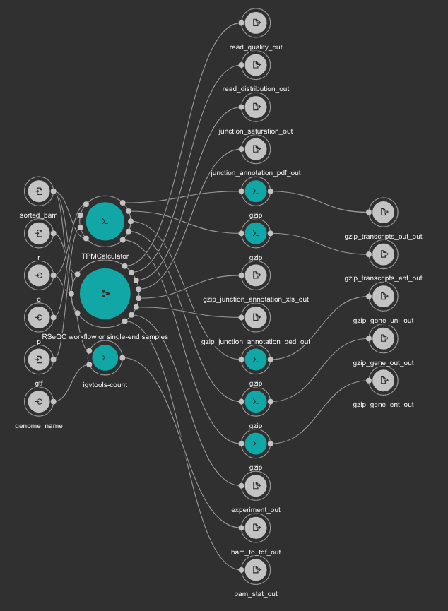
Inputs

• gtf: Genome GTF file. Variable GENOME_GTF in the Jupyter Notebooks. Type: File. Required.
• genome_name: Genome name as defined in IGV for TDF conversion. Type: string. Required.
• q: Minimum MAPQ value to use reads. We recommend 255. Type: int. Required.
• r: Reference Genome in BED format used by RSeQC. Variable GENOME_BED in the Jupyter Notebooks. Type: File. Required.
• sorted_bam: Sorted BAM file to quantify. Type: File. Required.

Outputs

• bam_to_tdf_out: TDF file created with igvtools from the BAM file for quick visualization. Type: File.
• gzip_gene_ent_out: TPMCalculator gene ENT output gzipped. Type: File.
• gzip_gene_out_out: TPMCalculator gene OUT output gzipped. Type: File.
• gzip_gene_uni_out: TPMCalculator gene UNI output gzipped. Type: File.
• gzip_transcripts_ent_out: TPMCalculator transcript ENT output gzipped. Type: File.
• gzip_transcripts_out_out: TPMCalculator transcript OUT output gzipped. Type: File.
• bam_stat_out: RSeQC BAM stats output. Type: File.
• experiment_out: RSeQC experiment output. Type: File.
• gzip_junction_annotation_bed_out: RSeQC junction annotation bed. Type: File.
• gzip_junction_annotation_xls_out: RSeQC junction annotation xls. Type: File.
• junction_annotation_pdf_out: RSeQC junction annotation PDF figure. Type: File.
• junction_saturation_out: RSeQC junction saturation output. Type: File.
• read_distribution_out: RSeQC read distribution output. Type: File.
• read_quality_out: RSeQC read quality output. Type: File.

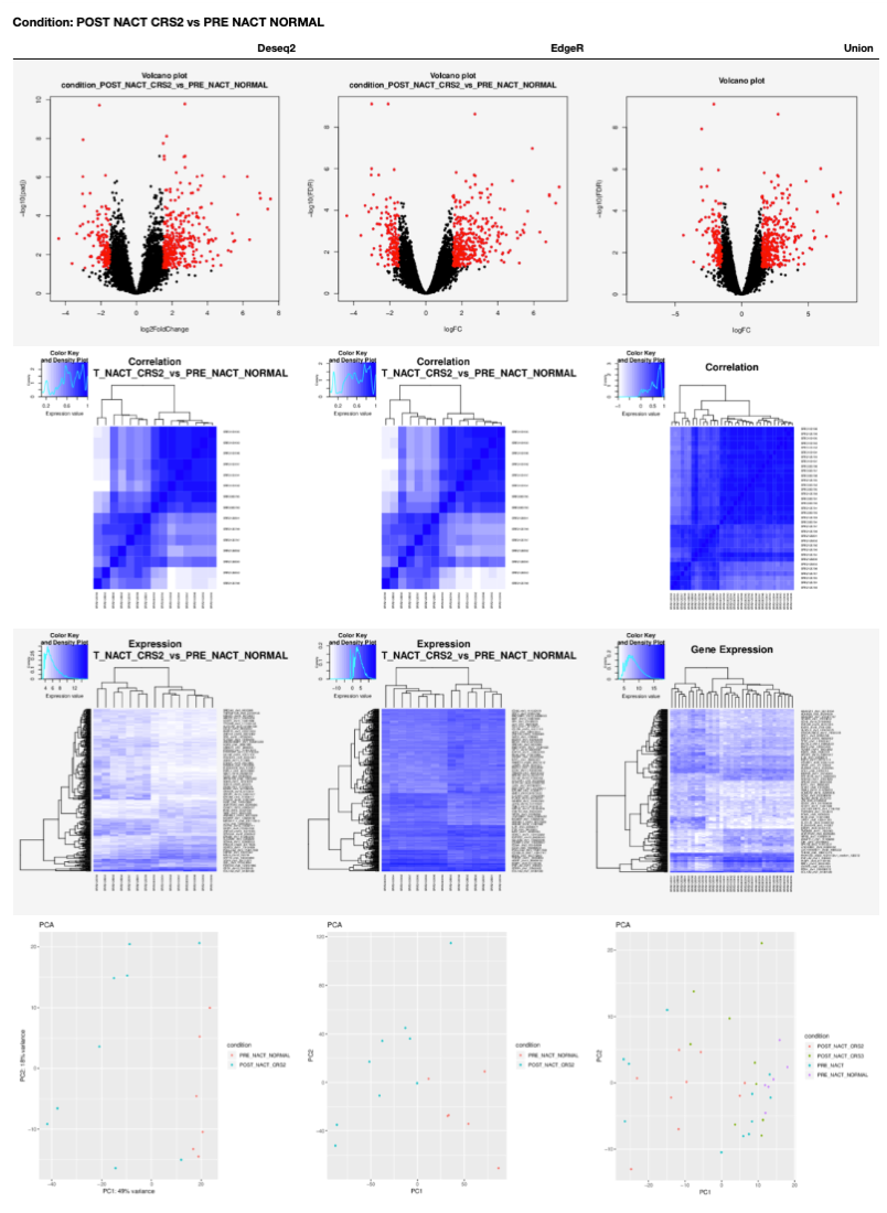
6.6.5. Differential Gene Expression analysis from RNA-Seq data

Our notebooks are designed to execute a Differential Gene Expression analysis using two available tools: DESeq2 and EdgeR. Also, the results for the interception of both tools output is reported with volcano plots, heatmaps and PCA plots.

The workflow use the sample_sheet.tsv file to generate an array with all combinations of conditions. The code to generate this array is very simple and can be found in the cell number 3 in the 05 - DGA.ipynb notebook.

comparisons = []
for s in itertools.combinations(factors['condition'].unique(), 2):
    comparisons.append(list(s))

Let's suppose we have a factors.txt file with three conditions: cond1, cond2 and cond3. The comparisons array will look like:

comparisons = [
    ['cond1', 'cond2'],
    ['cond1', 'cond3'],
    ['cond2', 'cond3']
]

To avoid this behavior and execute the comparison just in a set of conditions, you should remove the code in the cell number 3 in the 05 - DGA.ipynb notebook and manually create the array of combinations to be compared as:

comparisons = [
    ['cond1', 'cond3'],
]

The R code used for running DESeq2 is embedded in deseq2-2conditions.cwl from line 25 to line 169. The R code used for running EdgeR is embedded in edgeR-2conditions.cwl from line 25 to line 159.

A table with DGA plots is generated for each condition in the 00 - Project Report.ipynb as shown next.

6.6.6. GO enrichment from RNA-Seq data

The GO enrichment analysis is executed with an in-house developed python package named goenrichment. This tools uses the hypergeometric distribution test to estimate the probability of successes in selecting GO terms from a list of differentially expressed genes. The GO terms are represented as a network using the python library NetworkX.

The tool uses a pre-computed database, currently available for human and mouse, at https://ftp.ncbi.nlm.nih.gov/pub/goenrichment/. However, the project web page describe how to create your own database from a set of reference databases.

The workflow uses the factors.txt file to generate an array with all combinations of conditions. The code to generate this array is very simple and can be found in the cell number 3 in the 06 - GO enrichment.ipynb notebook.

comparisons = []
for s in itertools.combinations(factors['condition'].unique(), 2):
    comparisons.append(list(s))

Let's suppose we have a factors.txt file with three conditions: cond1, cond2 and cond3. The comparisons array will look like:

comparisons = [
    ['cond1', 'cond2'],
    ['cond1', 'cond3'],
    ['cond2', 'cond3']
]

To avoid this behavior and execute the comparison just in a set of conditions, you should remove the code in the cell number 3 in the 06 - GO enrichment.ipynb notebook and manually create the array of combinations to be compared as:

comparisons = [
    ['cond1', 'cond3'],
]

Additionally, the workflow requires three cutoff that are defined in the cell number 5 of the same notebook.

min_category_depth=4
min_category_size=3
max_category_size=500

Cutoffs definition

• min_category_depth: Min GO term graph depth to include in the report. Default: 4
• min_category_size: Min number of gene in a GO term to include in the report. Default: 3
• max_category_size: Max number of gene in a GO term to include in the report. Default: 500

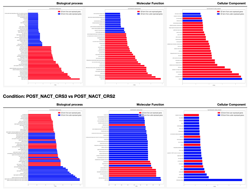
A table with GO terms plots is generated for each condition in the 00 - Project Report.ipynb as shown next. In these plots the red bars are for GO terms selected from the over expressed genes and the blue bars are for GO terms selected from the under expressed genes. It is important to clarify that the two sets of GO terms don't overlap each other.

6.7. Demo

PM4NGS includes a demo project that users can use to test the framework. It is pre-configured to use Docker as execution environment.

The RNASeq based demo process samples from the BioProject PRJNA290924.

Use this command to create the project structure in your local computer

localhost:~> pm4ngs-rnaseq-demo

Once it finish, start the jupyter server and execute the notebooks as it is indicated on them

localhost:~> jupyter notebook
[I 14:12:52.956 NotebookApp] Serving notebooks from local directory: /home/veraalva
[I 14:12:52.956 NotebookApp] Jupyter Notebook 6.1.4 is running at:
[I 14:12:52.956 NotebookApp] http://localhost:8888/?token=eae6a8d42ad12d6ace23f5d0923bcec14d0f798127750122
[I 14:12:52.956 NotebookApp]  or http://127.0.0.1:8888/?token=eae6a8d42ad12d6ace23f5d0923bcec14d0f798127750122
[I 14:12:52.956 NotebookApp] Use Control-C to stop this server and shut down all kernels (twice to skip confirmatio
n).
[C 14:12:52.959 NotebookApp]

    To access the notebook, open this file in a browser:
        file:///home/veraalva/.local/share/jupyter/runtime/nbserver-23251-open.html
    Or copy and paste one of these URLs:
        http://localhost:8888/?token=eae6a8d42ad12d6ace23f5d0923bcec14d0f798127750122
     or http://127.0.0.1:8888/?token=eae6a8d42ad12d6ace23f5d0923bcec14d0f798127750122

The results of this analysis is https://ftp.ncbi.nlm.nih.gov/pub/pm4ngs/examples/rnaseq-sra-paired/