7. Differential Binding detection from ChIP-Seq data
Differential binding analysis pipeline from ChIP-Seq data.
The workflow is comprised of five steps, as shown in next table. The first step, sample download and quality control, is for downloading samples from the NCBI SRA database, if necessary, or for executing the pre-processing quality control tools on all samples. Sample trimming and alignment are executed next. Post-processing quality control on ChIP-Seq samples is executed using Phantompeakqualtools, as recommended by the ENCODE consortia]. Then, a peak calling step is performed using MACS2, and peak annotation is executed with Homer. Peak reproducibility is explored with IDR. Finally, a differential binding analysis is completed with DiffBind.
| Step | Jupyter Notebook | Workflow CWL | Tool | Input | Output | CWL Tool |
|---|---|---|---|---|---|---|
| Sample Download and Quality Control | 01 - Pre-processing QC | download_quality_control.cwl | SRA-Tools | SRA accession | Fastq | fastq-dump.cwl |
| FastQC | Fastq | FastQC HTML and Zip | fastqc.cwl | |||
| Trimming | 02 - Samples trimming | Trimmomatic | Fastq | Fastq | ||
| Alignments and Quantification | 03 - Alignments | chip-seq-alignment.cwl | BWA | Fastq | BAM | bwa-mem.cwl |
| Samtools | SAM | BAM Sorted BAM BAM index BAM stats BAM flagstats |
||||
Peak Calling and IDR |
04 - Peak Calling and IDR | peak-calling-MACS2.cwl | IGVtools | Sorted BAM | TDF | igvtools-count.cw |
| MACS2 | tagAlign | Peaks (TSV), plots | macs2-callpeak.cwl | |||
| Homer | BAM | Annotation (TSV) FPKM values (TSV) | ||||
| IDR | Peaks | Peaks (TSV), plots | idr.cwl | |||
| Differential binding Analysis | 05 - Differential binding Detection | DiffBind | Read Matrix | Peaks (TSV), plots | diffBind.cwl |
7.1. Input requirements
The input requirement for the ChIPSeq pipeline is the Sample sheet file.
7.2. Pipeline command line
The ChIPSeq based project can be created using the following command line:
localhost:~> pm4ngs-chipseq
usage: Generate a PM4NGS project for ChIPSeq data analysis [-h] [-v]
                                                       --sample-sheet
                                                       SAMPLE_SHEET
                                                       [--config-file CONFIG_FILE]
                                                       [--copy-rawdata]
Options:
- sample-sheet: Sample sheet with the samples metadata
- config-file: YAML file with configuration for project creation
- copy-rawdata: Copy the raw data defined in the sample sheet to the project structure. (The data can be hosted locally or in an http server)
7.3. Creating the Differential Binding detection from ChIP-Seq data project
The pm4ngs-chipseq command line executed with the --sample-sheet option will let you type the different variables required for creating and configuring the project. The default value for each variable is shown in the brackets. After all questions are answered, the CWL workflow files will be cloned from the github repo ncbi/cwl-ngs-workflows-cbb to the folder bin/cwl.
localhost:~> pm4ngs-chipseq --sample-sheet my-sample-sheet.tsv
Generating ChIP-Seq data analysis project
author_name [Roberto Vera Alvarez]:
email [veraalva@ncbi.nlm.nih.gov]:
project_name [my_ngs_project]:
dataset_name [my_dataset_name]:
is_data_in_SRA [None]:
Select sequencing_technology:
1 - single-end
2 - paired-end
Choose from 1, 2 [1]: 2
create_demo [y]:
number_spots [1000000]:
organism [human]:
genome_name [hg38]:
genome_dir [hg38]:
aligner_index_dir [hg38/BWA]:
genome_fasta [hg38/genome.fa]:
genome_gtf [hg38/genome.gtf]:
genome_mappable_size [hg38]:
fdr [0.05]:
use_docker [y]:
max_number_threads [16]:
Cloning Git repo: https://github.com/ncbi/cwl-ngs-workflows-cbb to /Users/veraalva/my_ngs_project/bin/cwl
Updating CWLs dockerPull and SoftwareRequirement from: /Users/veraalva/my_ngs_project/requirements/conda-env-dependencies.yaml
bedtools with version 2.29.2 update image to: quay.io/biocontainers/bedtools:2.29.2--hc088bd4_0
    /Users/veraalva/my_ngs_project/bin/cwl/tools/bedtools/bedtools-docker.yml with old image replaced: quay.io/biocontainers/bedtools:2.28.0--hdf88d34_0
bioconductor-diffbind with version 2.16.0 update image to: quay.io/biocontainers/bioconductor-diffbind:2.16.0--r40h5f743cb_0
    /Users/veraalva/my_ngs_project/bin/cwl/tools/R/deseq2-pca.cwl with old image replaced: quay.io/biocontainers/bioconductor-diffbind:2.16.0--r40h5f743cb_2
    /Users/veraalva/my_ngs_project/bin/cwl/tools/R/macs-cutoff.cwl with old image replaced: quay.io/biocontainers/bioconductor-diffbind:2.16.0--r40h5f743cb_2
    /Users/veraalva/my_ngs_project/bin/cwl/tools/R/dga_heatmaps.cwl with old image replaced: quay.io/biocontainers/bioconductor-diffbind:2.16.0--r40h5f743cb_2
    /Users/veraalva/my_ngs_project/bin/cwl/tools/R/diffbind.cwl with old image replaced: quay.io/biocontainers/bioconductor-diffbind:2.16.0--r40h5f743cb_2
    /Users/veraalva/my_ngs_project/bin/cwl/tools/R/edgeR-2conditions.cwl with old image replaced: quay.io/biocontainers/bioconductor-diffbind:2.16.0--r40h5f743cb_2
    /Users/veraalva/my_ngs_project/bin/cwl/tools/R/volcano_plot.cwl with old image replaced: quay.io/biocontainers/bioconductor-diffbind:2.16.0--r40h5f743cb_2
    /Users/veraalva/my_ngs_project/bin/cwl/tools/R/readQC.cwl with old image replaced: quay.io/biocontainers/bioconductor-diffbind:2.16.0--r40h5f743cb_2
    /Users/veraalva/my_ngs_project/bin/cwl/tools/R/deseq2-2conditions.cwl with old image replaced: quay.io/biocontainers/bioconductor-diffbind:2.16.0--r40h5f743cb_2
bwa with version 0.7.17 update image to: quay.io/biocontainers/bwa:0.7.17--hed695b0_7
    /Users/veraalva/my_ngs_project/bin/cwl/tools/bwa/bwa-docker.yml with old image replaced: quay.io/biocontainers/bwa:0.7.17--h84994c4_5
homer with version 4.11 update image to: quay.io/biocontainers/homer:4.11--pl526h9a982cc_2
    /Users/veraalva/my_ngs_project/bin/cwl/tools/homer/homer-docker.yml with old image replaced: quay.io/biocontainers/homer:4.11--pl526h2bce143_2
Copying file /Users/veraalva/Work/Developer/Python/pm4ngs/pm4ngs-chipseq/example/pm4ngs_chipseq_demo_sample_data.csv  to /Users/veraalva/my_ngs_project/data/my_dataset_name/sample_table.csv
6 files loaded
Using table:
  sample_name file condition  replicate
0  SRR7549105             ES          1
1  SRR7549106             ES          2
2  SRR7549109            MEF          1
3  SRR7549110            MEF          2
4  SRR7549114             rB          1
5  SRR7549113             rB          2
 Done
The pm4ngs-chipseq command line will create a project structure as:
.
├── LICENSE
├── README.md
├── bin
│   └── cwl
├── config
│   └── init.py
├── data
│   └── my_dataset_name
├── doc
├── index.html
├── notebooks
│   ├── 00 - Project Report.ipynb
│   ├── 01 - Pre-processing QC.ipynb
│   ├── 02 - Samples trimming.ipynb
│   ├── 03 - Alignments.ipynb
│   ├── 04 - Peak Calling and IDR.ipynb
│   └── 05 - Differential binding Detection.ipynb
├── requirements
│   └── conda-env-dependencies.yaml
├── results
│   └── my_dataset_name
├── src
└── tmp

12 directories, 11 files
Note
ChIP-Seq based project variables
- author_name:
Default: [Roberto Vera Alvarez]
- email:
Default: [veraalva@ncbi.nlm.nih.gov]
- project_name:
Name of the project with no space nor especial characters. This will be used as project folder's name.
Default: [my_ngs_project]
- dataset_name:
Dataset to process name with no space nor especial characters. This will be used as folder name to group the data. This folder will be created under the data/{{dataset_name}} and results/{{dataset_name}}.
Default: [my_dataset_name]
- is_data_in_SRA:
If the data is in the SRA set this to y. A CWL workflow to download the data from the SRA database to the folder data/{{dataset_name}} and execute FastQC on it will be included in the 01 - Pre-processing QC.ipynb notebook.
Set this option to n, if the fastq files names and location are included in the sample sheet.
Default: [y]
- Select sequencing_technology:
Select one of the available sequencing technologies in your data.
Values: 1 - single-end, 2 - paired-end
- create_demo:
If the data is downloaded from the SRA and this option is set to y, only the number of spots specified in the next variable will be downloaded. Useful to test the workflow.
Default: [y]: y
- number_spots:
Number of sport to download from the SRA database. It is ignored is the create_demo is set to n.
Default: [1000000]
- organism:
Organism to process, e.g. human. This is used to link the selected genes to the NCBI gene database.
Default: [human]
- genome_name:
Genome name , e.g. hg38 or mm10.
Default: [hg38]
- genome_dir:
Absolute path to the directory with the genome annotation (genome.fa, genes.gtf) to be used by the workflow or the name of the genome.
If the name of the genome is used, PM4NGS will include a cell in the 03 - Alignments.ipynb notebook to download the genome files. The genome data will be at data/{{dataset_name}}/{{genome_name}}/
Default: [hg38]
- aligner_index_dir:
Absolute path to the directory with the genome indexes for BWA.
If {{genome_name}}/BWA is used, PM4NGS will include a cell in the 03 - Alignments.ipynb notebook to create the genome indexes for BWA.
Default: [hg38/BWA]
- genome_fasta:
Absolute path to the genome fasta file
If {{genome_name}}/genome.fa is used, PM4NGS will use the downloaded fasta file.
Default: [hg38/genome.fa]
- genome_gtf:
Absolute path to the genome GTF file
If {{genome_name}}/genes.gtf is used, PM4NGS will use the downloaded GTF file.
Default: [hg38/gene.gtf]
- genome_bed:
Absolute path to the genome BED file
If {{genome_name}}/genes.bed is used, PM4NGS will use the downloaded BED file.
Default: [hg38/genes.bed]
- genome_mappable_size:
Genome mappable size used by MACS. For human can be hg38 or in case of other genomes it is a number.
Default: [hg38]
- fdr:
Adjusted P-Value to be used as cutoff in the DG analysis, e.g. 0.05.
Default: [0.05]
- use_docker:
Set this to y if you will be using Docker. Otherwise Conda needs to be installed in the computer.
Default: [y]
- max_number_threads:
Number of threads available in the computer.
Default: [16]
7.4. Jupyter server
PM4NGS uses Jupyter as interface for users. After project creation the jupyter server should be started as shown below. The server will open a browser windows showing the project's structure just created.
localhost:~> jupyter notebook
7.5. Data processing
Start executing the notebooks from 01 to 05 waiting for each step completion. The 00 - Project Report.ipynb notebook can be executed after each notebooks to see the progress in the analysis.
7.6. CWL workflows
7.6.1. SRA download and QC workflow
This CWL workflow is designed to download FASTQ files from the NCBI SRA database using fastq-dump and then, execute fastqc generating a quality control report of the sample.
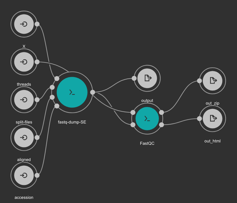
Inputs
- accession: SRA accession ID. Type: string. Required.
- aligned: Used it to download only aligned reads. Type: boolean. Optional.
- split-files: Dump each read into separate file. Files will receive suffix corresponding to read number. Type: boolean. Optional.
- threads: Number of threads. Type: int. Default: 1. Optional.
- X: Maximum spot id. Optional.
Outputs
- output: Fastq files downloaded. Type: File[]
- out_zip: FastQC report ZIP file. Type: File[]
- out_html: FastQC report HTML. Type: File[]
7.6.2. Samples Trimming
Our workflows uses Trimmomatic for read trimming. The Jupyter notebooks uses some basic Trimmomatic options that need to be modified depending on the FastQC quality control report generated for the sample.
7.6.3. BWA based alignment and quality control workflow
This workflow use BWA as base aligner. It also use SAMtools and bedtools for file conversion and statistics report. Finally, Phantompeakqualtools is used to generate quality control report for the processed samples.
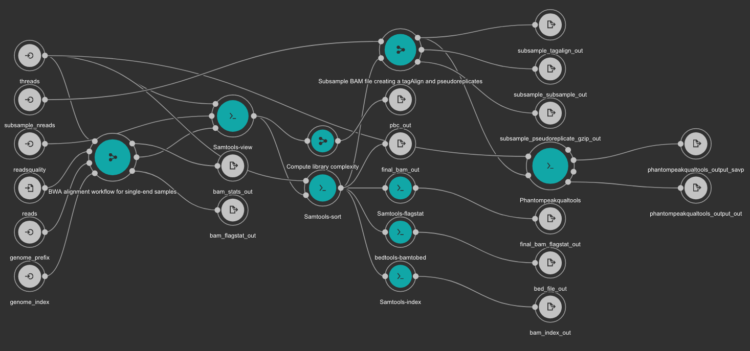
Inputs
- genome_index: Aligner indexes directory. Type: Directory. Required. Variable ALIGNER_INDEX in the Jupyter Notebooks.
- genome_prefix: Prefix of the aligner indexes. Generally, it is the name of the genome FASTA file. It can be used as os.path.basename(GENOME_FASTA) in the Jupyter Notebooks. Type: string. Required.
- readsquality: Minimum MAPQ value to use reads. We recommend for ChIP_exo dataa value of: 30. Type: int. Required.
- threads: Number of threads. Type: int. Default: 1. Optional.
- subsample_nreads: Number of reads to be used for the subsample. We recomend for ChIP_exo dataa value of: 500000. Type: int. Required.
- reads: FastQ file to be processed. Type: File. Required.
Outputs
- bam_flagstat_out: SAMtools flagstats for unfiltered BAM file. Type: File.
- bam_stats_out: SAMtools stats for unfiltered BAM file. Type: File.
- final_bam_flagstat_out: SAMtools flagstats for filtered BAM file. Type: File.
- bed_file_out:: Aligned reads in BED format. Type: File.
- final_bam_out: Final BAM file filtered and sorted. Type: File.
- bam_index_out: BAM index file. Type: File.
- pbc_out: Library complexity report. Type: File.
- phantompeakqualtools_output_out: Phantompeakqualtools main output. Type: File.
- phantompeakqualtools_output_savp: Phantompeakqualtools SAVP output. Type: File.
- subsample_pseudoreplicate_gzip_out: Subsample pseudoreplicates tagAlign gzipped. Type: File[].
- subsample_tagalign_out: Subsample tagAlign gzipped. Type: File[].
- subsample_subsample_out: Subsample shuffled tagAlign gzipped. Type: File[].
7.6.4. Peak caller workflow using MACS2
This workflow uses MACS2 as peak caller tool. The annotation is created using Homer and TDF files are created with igvtools.
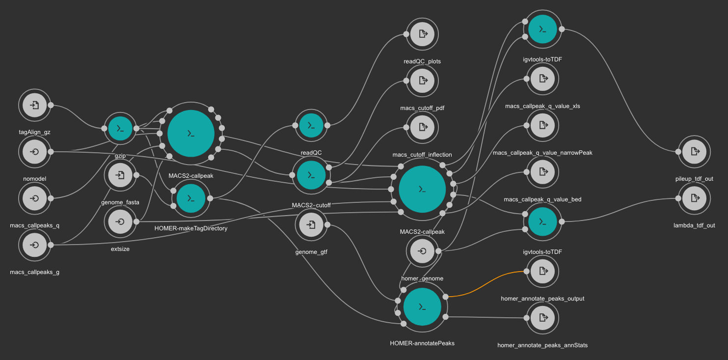
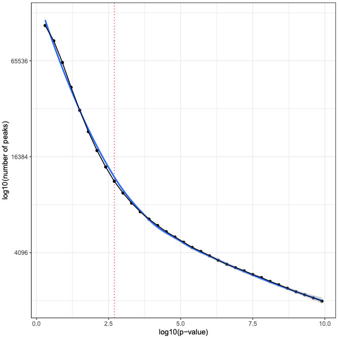
MACS2 is executed two times. First, the cutoff-analysis option is used to execute a cutoff value analysis which is used to estimate a proper value for the p-value used by MACS2 (for more detailed explanation read this thread).
RSeQC is also executed for quality control.
Inputs
- homer_genome: Homer genome name. Type: string. Required.
- genome_fasta Genome FASTA file. Type: File. Required. Variable GENOME_FASTA in the Jupyter Notebooks.
- genome_gtf: Genome GTF file. Type: File. Required. Variable GENOME_GTF in the Jupyter Notebooks.
- tagAlign_gz: Tag aligned file created with the BWA based alignment and quality control workflow. Type: File. Required.
- macs_callpeaks_g: Genome mapeable size as defined in MACS2. Type: string. Required. Variable GENOME_MAPPABLE_SIZE in the Jupyter Notebooks.
- macs_callpeaks_q: MACS2 q option. Starting qvalue (minimum FDR) cutoff to call significant regions. Type: float. Required. Variable fdr in the Jupyter Notebooks.
- nomodel: MACS2 nomodel option. MACS will bypass building the shifting model. Type: boolean. Optional.
- extsize: MACS2 extsize option. MACS uses this parameter to extend reads in 5'->3' direction to fix-sized fragments. Type: int. Optional.
Outputs
- readQC_plots: RSeQC plots. Type: File[]
- macs_cutoff_pdf MACS2 cutoff analysis plot in PDF format. Type: File
- macs_cutoff_inflection: MACS2 inflection q value used for the second round. Type: File
- macs_callpeak_q_value_narrowPeak: Final MACS2 narrowpeak file. Type: File
- macs_callpeak_q_value_xls: Final MACS2 XLS file. Type: File
- macs_callpeak_q_value_bed: Final MACS2 BED file. Type: File
- homer_annotate_peaks_output: Homer annotated BED file. Type: File
- homer_annotate_peaks_annStats: Homer annotation statistics. Type: File
- lambda_tdf_out: MACS2 lambda file in TDF format. Type: File
- pileup_tdf_out: MACS2 pileup file in TDF format. Type: File
7.6.5. MEME Motif detection workflow
Motif detection is executed using the MEME suite.
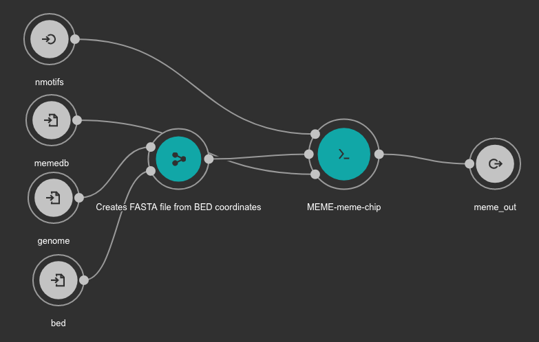
Inputs
- bed: BED file with detected peaks. Type: File. Required.
- memedb: MEME database for use by Tomtom and CentriMo. Type: File. Required.
- genome: Genome FASTA file. Variable GENOME_FASTA in the Jupyter Notebooks. Type: File. Required.
- nmotifs: Maximum number of motifs to find. We recommend use 10. Type: int. Required.
Outputs
- meme_out: MEME output directory. Type: Directory
7.6.6. MEME databases
MEME workflow depends on the MEME databases. Go to the MEME Suite Download page: http://meme-suite.org/doc/download.html
Download the latest version for the Motif Databases and GOMo Databases.
The downloaded files should be uncompressed in a directory data/meme. The final directory should be:
localhost:~> cd data
localhost:~> mkdir meme
localhost:~> cd meme
localhost:~> wget http://meme-suite.org/meme-software/Databases/motifs/motif_databases.12.18.tgz
localhost:~> wget http://meme-suite.org/meme-software/Databases/gomo/gomo_databases.3.2.tgz
localhost:~> tar xzf motif_databases.12.18.tgz
localhost:~> tar xzf gomo_databases.3.2.tgz
localhost:~> rm gomo_databases.3.2.tgz motif_databases.12.18.tgz
localhost:~> tree -d
.
├── gomo_databases
└── motif_databases
    ├── ARABD
    ├── CIS-BP
    ├── CISBP-RNA
    ├── ECOLI
    ├── EUKARYOTE
    ├── FLY
    ├── HUMAN
    ├── JASPAR
    ├── MALARIA
    ├── MIRBASE
    ├── MOUSE
    ├── PROKARYOTE
    ├── PROTEIN
    ├── RNA
    ├── TFBSshape
    ├── WORM
    └── YEAST

19 directories
See also an example in our test project: https://ftp.ncbi.nlm.nih.gov/pub/pm4ngs/examples/chipexo-single/data/
7.6.7. Differential binding analysis with Diffbind
Differential binding event is detected with Diffbind. Thsi tool will be executed for all comparisons added to the comparisons array. See cell number 3 in the notebook 05 - Differential binding analysis.ipynb (ChIP-Seq workflow).
Inputs
- bamDir: Directory with the BAM files. Type: Directory. Required.
- bedDir: Directory with BED files created from MACS2 peak calling workflow Type: Directory. Required.
Outputs
- outpng: PNG files created from Diffbind. Type File[]
- outxls: XLS files created from Diffbind. Type: File[]
- outbed BED files created from Diffbind. Type: File[]
7.7. Demo
PM4NGS includes a demo project that users can use to test the framework. It is pre-configured to use Docker as execution environment.
The ChIPSeq based demo process samples from the BioProject PRJNA481982.
Use this command to create the project structure in your local computer
localhost:~> pm4ngs-chipseq-demo
Once it finish, start the jupyter server and execute the notebooks as it is indicated on them
localhost:~> jupyter notebook
[I 14:12:52.956 NotebookApp] Serving notebooks from local directory: /home/veraalva
[I 14:12:52.956 NotebookApp] Jupyter Notebook 6.1.4 is running at:
[I 14:12:52.956 NotebookApp] http://localhost:8888/?token=eae6a8d42ad12d6ace23f5d0923bcec14d0f798127750122
[I 14:12:52.956 NotebookApp]  or http://127.0.0.1:8888/?token=eae6a8d42ad12d6ace23f5d0923bcec14d0f798127750122
[I 14:12:52.956 NotebookApp] Use Control-C to stop this server and shut down all kernels (twice to skip confirmatio
n).
[C 14:12:52.959 NotebookApp]

    To access the notebook, open this file in a browser:
        file:///home/veraalva/.local/share/jupyter/runtime/nbserver-23251-open.html
    Or copy and paste one of these URLs:
        http://localhost:8888/?token=eae6a8d42ad12d6ace23f5d0923bcec14d0f798127750122
     or http://127.0.0.1:8888/?token=eae6a8d42ad12d6ace23f5d0923bcec14d0f798127750122
The results of this analysis is https://ftp.ncbi.nlm.nih.gov/pub/pm4ngs/examples/chipseq-hmgn1/