Differential Gene expression from RNA-Seq data

Warning

Read the Background Information before proceeding with these steps

Warning

Read the Project Templates Installation notes to have the cookiecutter available in you shell depending on the execution environment you will be using.

Samples description file

A TSV file named factors.txt is the main file for the projects and workflow. This file should be created before any project creation. It is the base of the workflow and should be copied to the folder data/{{dataset_name}} just after creating the project structure.

The initial sample names, file name prefixes and metadata are specified on it.

It should have the following columns:

id	SampleID	condition	replicate
classical01	SRR4053795	classical	1
classical01	SRR4053796	classical	2
nonclassical01	SRR4053802	nonclassical	1
nonclassical01	SRR4053803	nonclassical	2

Warning

Columns names are required and are case sensitive.

Columns

• id: Sample names. It can be different of sample file name.

• SampleID: This is the prefix of the sample file name.

  For single-end data the prefix ends in the file extension. In this case, for the first column, a file name named SRR4053795.fastq.gz must exist.

  For paired-end data the files SRR4053795_1.fastq.gz and SRR4053795_2.fastq.gz must exist.

  The data files should be copied to the folder data/{{dataset_name}}/.

• condition: Conditions to analyze or group the samples. Avoid using non alphanumeric characters.

  For RNASeq projects the differential gene expression will be generated comparing these conditions. If there are multiple conditions all comparisons will be generated. It must be at least two conditions.

  For ChIPSeq projects differential binding events will be detected comparing these conditions. If there are multiple conditions all comparisons will be generated. It must be at least two conditions.

  For ChIPexo projects the samples of the same condition will be grouped for the peak calling with MACE.

• replicate: Replicate number for samples.

Installation

RNA-Seq workflow with Conda/Bioconda

The RNA-Seq project structure is created using the conda environment named templates.

First step is to activate the templates environment:

localhost:~> conda activate templates

Then, a YAML file (for this example I will call this file: rnaseq-sra-paired.yaml) with your project detail should be created.

default_context:
  author_name: "Roberto Vera Alvarez"
  user_email: "veraalva@ncbi.nlm.nih.gov"
  project_name: "rnaseq-sra-paired"
  dataset_name: "PRJNA290924"
  is_data_in_SRA: "y"
  ngs_data_type: "RNA-Seq"
  sequencing_technology: "paired-end"
  create_demo: "y"
  number_spots: "1000000"
  organism: "human"
  genome_dir: "/gfs/data/genomes/igenomes/Homo_sapiens/UCSC/hg38"
  genome_name: "hg38"
  aligner_index_dir: "{{ cookiecutter.genome_dir}}/STAR"
  genome_fasta: "{{ cookiecutter.genome_dir}}/genome.fa"
  genome_gtf: "{{ cookiecutter.genome_dir}}/genes.gtf"
  genome_gff: "{{ cookiecutter.genome_dir}}/genes.gff"
  genome_gff3: "{{ cookiecutter.genome_dir}}/genes.gff3"
  genome_bed: "{{ cookiecutter.genome_dir}}/genes.bed"
  genome_chromsizes: "{{ cookiecutter.genome_dir}}/chrom.sizes"
  genome_mappable_size: "hg38"
  genome_blacklist: "{{ cookiecutter.genome_dir}}/hg38-blacklist.bed"
  fold_change: "2.0"
  fdr: "0.05"
  use_docker: "n"
  pull_images: "n"
  use_conda: "y"
  cwl_runner: "cwl-runner"
  cwl_workflow_repo: "https://github.com/ncbi/cwl-ngs-workflows-cbb"
  create_virtualenv: "n"
  use_gnu_parallel: "y"
  max_number_threads: "16"

A full description of this parameters are here.

After the rnaseq-sra-paired.yaml is created the project structure should be created using this command obtaining the following output.

localhost:~> cookiecutter --no-input --config-file rnaseq-sra-paired.yaml https://github.com/ncbi/pm4ngs.git
Checking RNA-Seq workflow dependencies .......... Done
localhost:~>

This process should create a project organizational structure like this:

localhost:~> tree rnaseq-sra-paired
rnaseq-sra-paired
├── bin
│   ├── bioconda (This directory include a conda envs for all bioinfo tools)
│   ├── cwl-ngs-workflows-cbb (CWL workflow repo cloned here)
│   └── jupyter (This directory include a conda envs for Jupyter notebooks)
├── config
│   └── init.py
├── data
│   └── PRJNA290924
├── doc
├── index.html
├── LICENSE
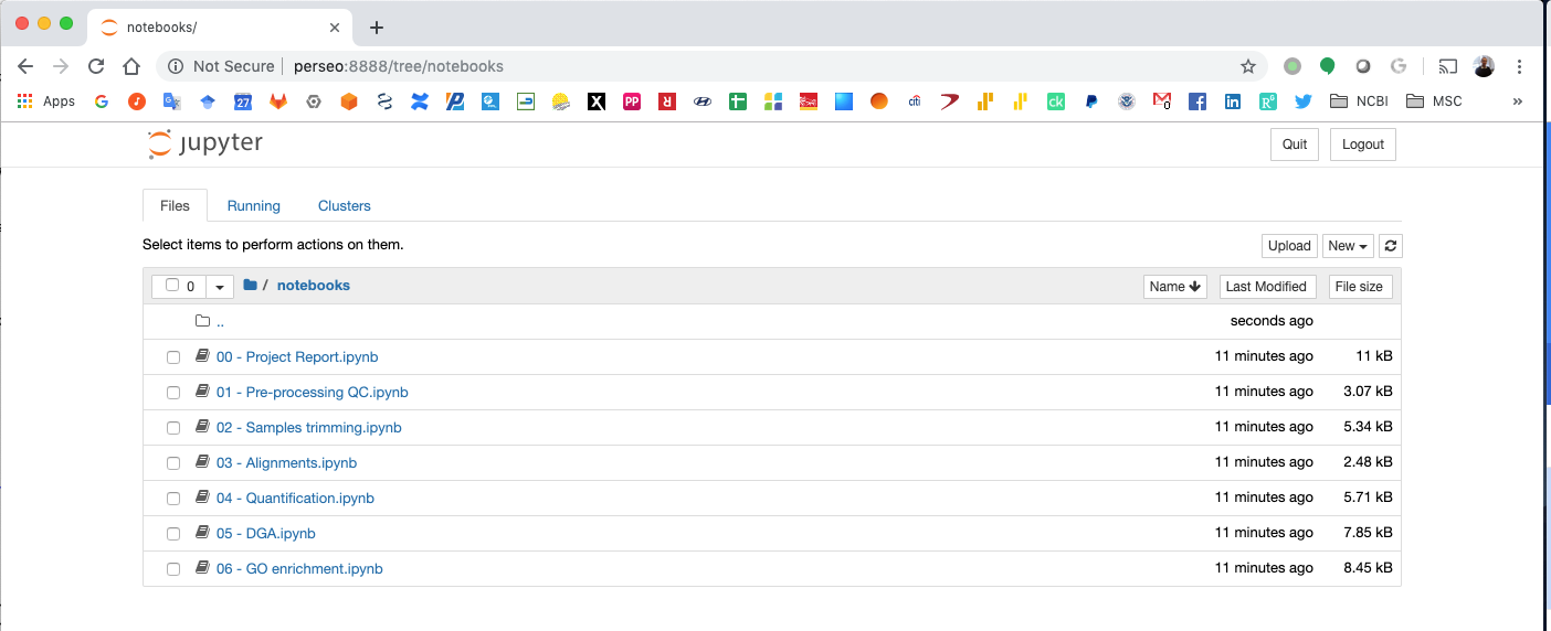
├── notebooks
│   ├── 00 - Project Report.ipynb
│   ├── 01 - Pre-processing QC.ipynb
│   ├── 02 - Samples trimming.ipynb
│   ├── 03 - Alignments.ipynb
│   ├── 04 - Quantification.ipynb
│   ├── 05 - DGA.ipynb
│   └── 06 - GO enrichment.ipynb
├── README.md
├── requirements
│   └── python.txt
├── results
│   └── PRJNA290924
├── src
└── tmp

14 directories, 12 files

Now you should copied the factors.txt file to the folder: data/PRJNA290924.

After this process, cookiecutter should have created create two virtual environment for this workflow.

The first one is for running the Jupyter notebooks which require Python 3.6+ and it is named: jupyter. It can be manually installed as described in here.

The second environment is be used to install all Bioinformatics tools required by the workflow and it will be named: bioconda.

You can verify the environments running this command:

localhost:~> conda env list
# conda environments:
#
base                  *  /gfs/conda
tempates                 /gfs/conda/envs/templates
                         /home/veraalva/rnaseq-sra-paired/bin/bioconda
                         /home/veraalva/rnaseq-sra-paired/bin/jupyter

localhost:~>

Please, note that the Conda prefix /gfs/conda will be different in you host. Also, note that the bioconda and jupyter envs are inside the bin directory of your project keeping them static inside the project organizational structure.

RNA-Seq workflow usage with Conda/Bioconda

For start using the workflow you need to activate the conda environments bioconda and jupyter.

localhost:~> conda activate /home/veraalva/rnaseq-sra-paired/bin/bioconda
localhost:~> conda activate --stack /home/veraalva/rnaseq-sra-paired/bin/jupyter

Note the --stack option to have both environment working at the same time. Also, the order is important, bioconda should be activated before jupyter.

Test the conda envs:

localhost:~> which fastqc
/home/veraalva/rnaseq-sra-paired/bin/bioconda/bin/fastqc
localhost:~> which jupyter
/home/veraalva/rnaseq-sra-paired/bin/jupyter/bin/jupyter

Note that the fastqc tools is installed in the bioconda env and the jupyter command is installed in the jupyter env.

Then, you can start the jupyter notebooks.

localhost:~> jupyter notebook

If the workflow is deployed in a remote machine using SSH access the correct way to start the notebooks is:

localhost:~> jupyter notebook --no-browser --ip='0.0.0.0'

In this case the option --ip='0.0.0.0' will server the Jupyter notebook on all network interfaces and you can access them from your desktop browser using the port returned by the Jupyter server.

Finally, you should navegate in your browser to the notebooks folder and start executing all notebooks by their order leaving the 00 - Project Report.ipynb to the end.

RNA-Seq workflow with Docker

In this case, the RNA-Seq project structure is created using the Python virtual environment as described here

First step is to activate the Python virtual environment.

localhost:~> source venv-templates/bin/activate

Then, a YAML file (for this example I will call this file: rnaseq-sra-paired.yaml) with your project detail should be created.

default_context:
  author_name: "Roberto Vera Alvarez"
  user_email: "veraalva@ncbi.nlm.nih.gov"
  project_name: "rnaseq-sra-paired"
  dataset_name: "PRJNA290924"
  is_data_in_SRA: "y"
  ngs_data_type: "RNA-Seq"
  sequencing_technology: "paired-end"
  create_demo: "y"
  number_spots: "1000000"
  organism: "human"
  genome_dir: "/gfs/data/genomes/igenomes/Homo_sapiens/UCSC/hg38"
  genome_name: "hg38"
  aligner_index_dir: "{{ cookiecutter.genome_dir}}/STAR"
  genome_fasta: "{{ cookiecutter.genome_dir}}/genome.fa"
  genome_gtf: "{{ cookiecutter.genome_dir}}/genes.gtf"
  genome_gff: "{{ cookiecutter.genome_dir}}/genes.gff"
  genome_gff3: "{{ cookiecutter.genome_dir}}/genes.gff3"
  genome_bed: "{{ cookiecutter.genome_dir}}/genes.bed"
  genome_chromsizes: "{{ cookiecutter.genome_dir}}/chrom.sizes"
  genome_mappable_size: "hg38"
  genome_blacklist: "{{ cookiecutter.genome_dir}}/hg38-blacklist.bed"
  fold_change: "2.0"
  fdr: "0.05"
  use_docker: "y"
  pull_images: "y"
  use_conda: "n"
  cwl_runner: "cwl-runner"
  cwl_workflow_repo: "https://github.com/ncbi/cwl-ngs-workflows-cbb"
  create_virtualenv: "y"
  use_gnu_parallel: "y"
  max_number_threads: "16"

A full description of this parameters are here.

After the rnaseq-sra-paired.yaml is created the project structure should be created using this command obtaining the following output.

localhost:~> cookiecutter --no-input --config-file rnaseq-sra-paired.yaml https://github.com/ncbi/pm4ngs.git
Cloning Git repo: https://github.com/ncbi/cwl-ngs-workflows-cbb to /home/veraalva/rnaseq-sra-paired/bin/cwl-ngs-workflows-cbb
Creating a Python3.7 virtualenv
Installing packages in: /home/veraalva/rnaseq-sra-paired/venv using file /home/veraalva/rnaseq-sra-paired/requirements/python.txt
Checking RNA-Seq workflow dependencies .
    Pulling image: quay.io/biocontainers/fastqc:0.11.8--1 . Done .
    Pulling image: quay.io/biocontainers/trimmomatic:0.39--1 . Done .
    Pulling image: quay.io/biocontainers/star:2.7.1a--0 . Done .
    Pulling image: quay.io/biocontainers/samtools:1.9--h91753b0_8 . Done .
    Pulling image: quay.io/biocontainers/rseqc:3.0.0--py_3 . Done .
    Pulling image: quay.io/biocontainers/tpmcalculator:0.0.3--hdbb99b9_0 . Done .
    Pulling image: quay.io/biocontainers/igvtools:2.5.3--0 . Done .
    Pulling image: quay.io/biocontainers/sra-tools:2.9.6--hf484d3e_0 . Done .
    Pulling image: ubuntu:18.04 . Done
    Building image: r-3.5_ubuntu-18.04 . Done  Done
localhost:~>

This process should create a project organizational structure like this:

localhost:~> tree rnaseq-sra-paired
rnaseq-sra-paired
├── bin
│   └── cwl-ngs-workflows-cbb (CWL workflow repo cloned here)
├── config
│   └── init.py
├── data
│   └── PRJNA290924
├── doc
├── index.html
├── LICENSE
├── notebooks
│   ├── 00 - Project Report.ipynb
│   ├── 01 - Pre-processing QC.ipynb
│   ├── 02 - Samples trimming.ipynb
│   ├── 03 - Alignments.ipynb
│   ├── 04 - Quantification.ipynb
│   ├── 05 - DGA.ipynb
│   └── 06 - GO enrichment.ipynb
├── README.md
├── requirements
│   └── python.txt
├── results
│   └── PRJNA290924
├── src
├── tmp
└── venv
    ├── bin
    ├── etc
    ├── include
    ├── lib
    ├── locale
    ├── README.rst
    └── share

19 directories, 13 files

Now you should copied the factors.txt file to the directory: data/PRJNA238004.

After this process, cookiecutter should have pulled all docker images require by the project.

RNA-Seq workflow usage with Docker

For start using the workflow you need to activate the Python environment inside the project.

localhost:~> source venv/bin/activate

Then, you can start the jupyter notebooks now.

localhost:~> jupyter notebook

If the workflow is deployed in a remote machine using SSH access the correct way to start the notebooks is:

localhost:~> jupyter notebook --no-browser --ip='0.0.0.0'

In this case the option --ip='0.0.0.0' will server the Jupyter notebook on all network interfaces and you can access them from your desktop browser using the port returned by the Jupyter server.

Finally, you should navigate in your browser to the notebooks directory and start executing all notebooks by their order leaving the 00 - Project Report.ipynb to the end.

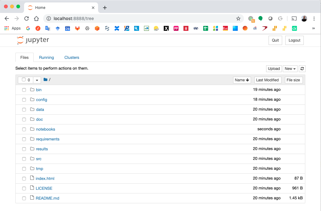
Jupyter Notebook Server

Top-level directories from the Jupyter server viewed in a web browser

Notebook generated fro the Chip-exo data analysis

CWL workflows

SRA download and QC workflow

This CWL workflow is designed to download FASTQ files from the NCBI SRA database using fastq-dump and then, execute fastqc generating a quality control report of the sample.

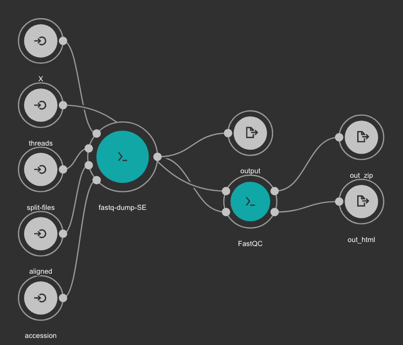
Inputs

• accession: SRA accession ID. Type: string. Required.

• aligned: Used it to download only aligned reads. Type: boolean. Optional.

• split-files: Dump each read into separate file. Files will receive suffix corresponding to read number. Type: boolean. Optional.

• threads: Number of threads. Type: int. Default: 1. Optional.

• X: Maximum spot id. Optional.

Outputs

• output: Fastq files downloaded. Type: File[]

• out_zip: FastQC report ZIP file. Type: File[]

• out_html: FastQC report HTML. Type: File[]

Samples Trimming

Our workflows uses Trimmomatic for read trimming. The Jupyter notebooks uses some basic Trimmomatic options that need to be modified depending on the FastQC quality control report generated for the sample.

STAR based alignment and sorting

This workflows use STAR for alignning RNA-Seq reads to a genome. The obtained BAM file is sorted using SAMtools. Statistics outputs from STAR and SAMtools are returned as well.

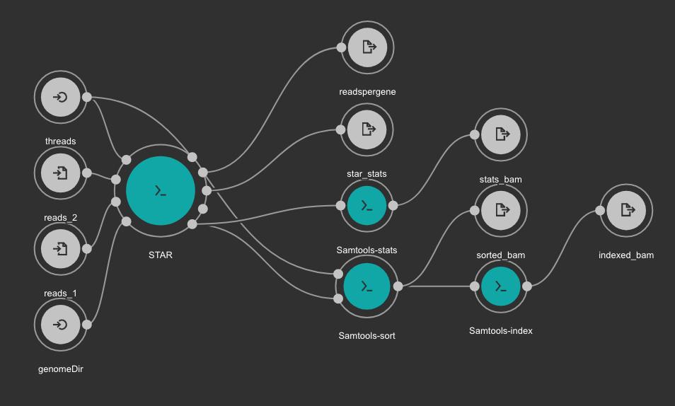
Inputs

• genomeDir: Aligner indexes directory. Type: Directory. Required. Variable ALIGNER_INDEX in the Jupyter Notebooks.

• threads: Number of threads. Type: int. Default: 1. Optional.

• reads_1: FastQ file to be processed for paired-end reads _1. Type: File. Required.

• reads_2: FastQ file to be processed for paired-end reads _2. Type: File. Required.

Outputs

• sorted_bam: Final BAM file filtered and sorted. Type: File.

• indexed_bam: BAM index file. Type: File.

• star_stats: STAR alignment statistics. Type: File.

• readspergene: STAR reads per gene output. Type: File.

• stats_bam: SAMtools stats output: Type: File.

RNA-Seq quantification and QC workflow using TPMCalculator

This workflow uses TPMCalculator to quantify the abundance of genes and transcripts from the sorted BAM file. Additionally, RSeQC is executed to generate multiple quality control outputs from the sorted BAM file. At the end, a TDF file is generated using igvtools from the BAM file for a quick visualization.

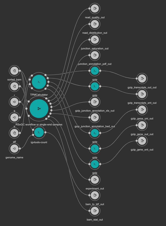
Inputs

• gtf: Genome GTF file. Variable GENOME_GTF in the Jupyter Notebooks. Type: File. Required.

• genome_name: Genome name as defined in IGV for TDF conversion. Type: string. Required.

• q: Minimum MAPQ value to use reads. We recommend 255. Type: int. Required.

• r: Reference Genome in BED format used by RSeQC. Variable GENOME_BED in the Jupyter Notebooks. Type: File. Required.

• sorted_bam: Sorted BAM file to quantify. Type: File. Required.

Outputs

• bam_to_tdf_out: TDF file created with igvtools from the BAM file for quick visualization. Type: File.

• gzip_gene_ent_out: TPMCalculator gene ENT output gzipped. Type: File.

• gzip_gene_out_out: TPMCalculator gene OUT output gzipped. Type: File.

• gzip_gene_uni_out: TPMCalculator gene UNI output gzipped. Type: File.

• gzip_transcripts_ent_out: TPMCalculator transcript ENT output gzipped. Type: File.

• gzip_transcripts_out_out: TPMCalculator transcript OUT output gzipped. Type: File.

• bam_stat_out: RSeQC BAM stats output. Type: File.

• experiment_out: RSeQC experiment output. Type: File.

• gzip_junction_annotation_bed_out: RSeQC junction annotation bed. Type: File.

• gzip_junction_annotation_xls_out: RSeQC junction annotation xls. Type: File.

• junction_annotation_pdf_out: RSeQC junction annotation PDF figure. Type: File.

• junction_saturation_out: RSeQC junction saturation output. Type: File.

• read_distribution_out: RSeQC read distribution output. Type: File.

• read_quality_out: RSeQC read quality output. Type: File.

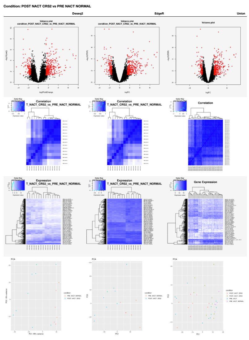
Differential Gene Expression analysis from RNA-Seq data

Our notebooks are designed to execute a Differential Gene Expression analysis using two available tools: DESeq2 and EdgeR. Also, the results for the interception of both tools output is reported with volcano plots, heatmaps and PCA plots.

The workflow use the factors.txt file to generate an array with all combinations of conditions. The code to generate this array is very simple and can be found in the cell number 3 in the 05 - DGA.ipynb notebook.

comparisons = []
for s in itertools.combinations(factors['condition'].unique(), 2):
    comparisons.append(list(s))

Let's suppose we have a factors.txt file with three conditions: cond1, cond2 and cond3. The comparisons array will look like:

comparisons = [
    ['cond1', 'cond2'],
    ['cond1', 'cond3'],
    ['cond2', 'cond3']
]

To avoid this behavior and execute the comparison just in a set of conditions, you should remove the code in the cell number 3 in the 05 - DGA.ipynb notebook and manually create the array of combinations to be compared as:

comparisons = [
    ['cond1', 'cond3'],
]

The R code used for running DESeq2 is embedded in deseq2-2conditions.cwl from line 14 to line 178. The R code used for running EdgeR is embedded in edgeR-2conditions.cwl from line 14 to line 165.

A table with DGA plots is generated for each condition in the 00 - Project Report.ipynb as shown next.

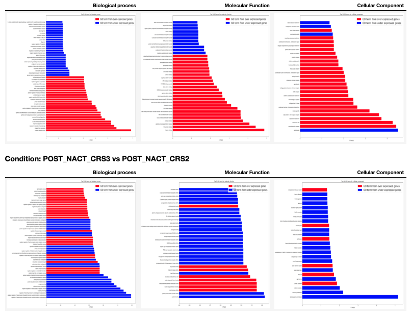
GO enrichment from RNA-Seq data

The GO enrichment analysis is executed with an in-house developed python package named goenrichment. This tools uses the hypergeometric distribution test to estimate the probability of successes in selecting GO terms from a list of differentially expressed genes. The GO terms are represented as a network using the python library NetworkX.

The tool uses a pre-computed database, currently available for human and mouse, at https://ftp.ncbi.nlm.nih.gov/pub/goenrichment/. However, the project web page describe how to create your own database from a set of reference databases.

The workflow uses the factors.txt file to generate an array with all combinations of conditions. The code to generate this array is very simple and can be found in the cell number 3 in the 06 - GO enrichment.ipynb notebook.

comparisons = []
for s in itertools.combinations(factors['condition'].unique(), 2):
    comparisons.append(list(s))

Let's suppose we have a factors.txt file with three conditions: cond1, cond2 and cond3. The comparisons array will look like:

comparisons = [
    ['cond1', 'cond2'],
    ['cond1', 'cond3'],
    ['cond2', 'cond3']
]

To avoid this behavior and execute the comparison just in a set of conditions, you should remove the code in the cell number 3 in the 06 - GO enrichment.ipynb notebook and manually create the array of combinations to be compared as:

comparisons = [
    ['cond1', 'cond3'],
]

Additionally, the workflow requires three cutoff that are defined in the cell number 5 of the same notebook.

min_category_depth=4
min_category_size=3
max_category_size=500

Cutoffs definition

• min_category_depth: Min GO term graph depth to include in the report. Default: 4

• min_category_size: Min number of gene in a GO term to include in the report. Default: 3

• max_category_size: Max number of gene in a GO term to include in the report. Default: 500

A table with GO terms plots is generated for each condition in the 00 - Project Report.ipynb as shown next. In these plots the red bars are for GO terms selected from the over expressed genes and the blue bars are for GO terms selected from the under expressed genes. It is important to clarify that the two sets of GO terms don't overlap each other.

Test Project

A test project is available (read-only) at https://ftp.ncbi.nlm.nih.gov/pub/pm4ngs/examples/rnaseq-sra-paired

Extra requirements

Creating STAR indexes

This workflow uses STAR for sequence alignment. The STAR index creation is not included in the workflow, that's why we are including an small section here to describe how the STAR indexes can be created.

The genome.fa and genes.gtf files should be copied to the genome directory.

localhost:~> conda activate /home/veraalva/rnaseq-sra-paired/bin/bioconda
localhost:~> conda activate --stack /home/veraalva/rnaseq-sra-paired/bin/jupyter
localhost:~> cd rnaseq-sra-paired/data
localhost:~> mkdir genome
localhost:~> cd genome
localhost:~> mkdir STAR
localhost:~> cd STAR
localhost:~> cwl-runner --no-container ../../../bin/cwl-ngs-workflows-cbb/tools/STAR/star-index.cwl --runThreadN 16 --genomeDir . --genomeFastaFiles ../genome.fa  --sjdbGTFfile ../genes.gtf
localhost:~> cd ..
localhost:~> tree
.
├── genes.gtf
├── genome.fa
└── STAR
    ├── chrLength.txt
    ├── chrNameLength.txt
    ├── chrName.txt
    ├── chrStart.txt
    ├── exonGeTrInfo.tab
    ├── exonInfo.tab
    ├── geneInfo.tab
    ├── Genome
    ├── genomeParameters.txt
    ├── Log.out
    ├── SA
    ├── SAindex
    ├── sjdbInfo.txt
    ├── sjdbList.fromGTF.out.tab
    ├── sjdbList.out.tab
    └── transcriptInfo.tab

1 directory, 18 files

Here all files inside the directory STAR are created by the workflow.

Creating BED files from GTF

For generating a BED file from a GTF.

The genes.gtf file should be copied to the genome directory.

localhost:~> conda activate /home/veraalva/rnaseq-sra-paired/bin/bioconda
localhost:~> conda activate --stack /home/veraalva/rnaseq-sra-paired/bin/jupyter
localhost:~> cd rnaseq-sra-paired/data
localhost:~> mkdir genome
localhost:~> cd genome
localhost:~> cwl-runner --no-container ../../bin/cwl-ngs-workflows-cbb/workflows/UCSC/gtftobed.cwl --gtf genes.gtf
localhost:~> tree
.
├── genes.bed
├── genes.genePred
├── genes.gtf
└── genome.fa

0 directory, 4 files

Here the files genes.bed and genes.genePred are created from the workflow.